DIGLM on Higgs dataset

In this notebook we train the DIGLM model on the dataset HIGGS.csv from UCI Machine Learning Repository.

This notebook is divided essentially in five parts:

1. Downloading and preparing (slicing) the dataset
2. Plotting features (to get an initial idea)
3. Initializing the model
4. Fitting and evaluating performances
5. Plotting results

Package needed

try:
    import google.colab
    IN_COLAB = True
except:
    IN_COLAB = False
if IN_COLAB:
    !git clone https://github.com/MarcoRiggirello/diglm

import sys
import os

sys.path.append('diglm/src')
sys.path.append('../../../src')

import logging

# sinlencing tensorflow warnings
os.environ['TF_CPP_MIN_LOG_LEVEL'] = '3'
logging.getLogger('tensorflow').setLevel(logging.FATAL)

import numpy as np
import pandas as pd
import seaborn as sns
from matplotlib import pyplot as plt
import imageio
from PIL import Image

import tensorflow as tf
from tensorflow_probability import distributions as tfd
from tensorflow_probability import glm as tfglm
from tensorflow_probability import bijectors as tfb
from tensorflow.keras import metrics

from spqr import NeuralSplineFlow as NSF
from diglm import Diglm

from download import download_file

Downloading data

To download the dataset we use the function download_file in the download.py module: it will check if the dataset already exists in the current directory or download it from the internet.

url = 'https://archive.ics.uci.edu/ml/machine-learning-databases/00280/HIGGS.csv.gz'
file_path = os.path.join('../model_test/download/HIGGS.csv.gz')
download_file(url, file_path)

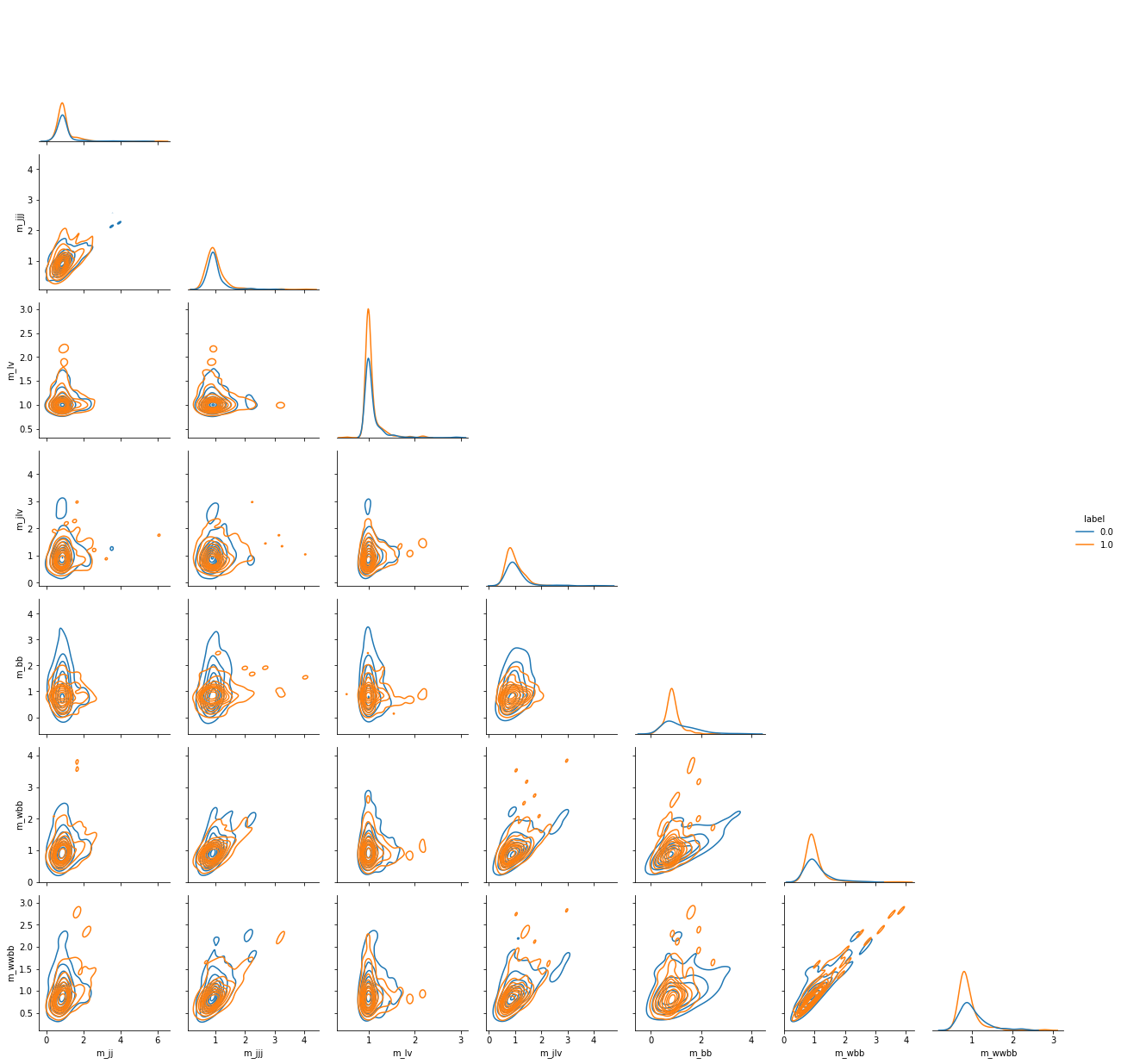
Plotting features of the dataset

We use seaborn to display scatterplot matrices of the correlation between features in the dataset.

column_labels = ['label','lepton pT', 'lepton eta', 'lepton phi',
                 'missing energy magnitude', 'missing energy phi',
                 'jet 1 pt', 'jet 1 eta', 'jet 1 phi',
                 'jet 1 b-tag', 'jet 2 pt', 'jet 2 eta',
                 'jet 2 phi', 'jet 2 b-tag', 'jet 3 pt',
                 'jet 3 eta', 'jet 3 phi', 'jet 3 b-tag',
                 'jet 4 pt', 'jet 4 eta', 'jet 4 phi',
                 'jet 4 b-tag', 'm_jj', 'm_jjj','m_lv',
                 'm_jlv', 'm_bb', 'm_wbb', 'm_wwbb']
data = pd.read_csv(file_path,
                   header=0,
                   names=column_labels,
                   nrows=8192*128)

grid = sns.PairGrid(data.head(500),
                    hue='label',
                    vars=column_labels[22:],
                    corner=True)
grid.map_diag(sns.kdeplot)
grid.map_offdiag(sns.kdeplot)
grid.add_legend()

<seaborn.axisgrid.PairGrid at 0x7f28b82a9960>

Slicing data: train, validation, test

We slice the dataframe to obtain train, validation and test samples (there are 11 milion examples complessively). Data appear to have mixed labels already, so that a simple slicing is sufficient to obtain good sampling.

BATCH_SIZE = 1024
TRAIN_SIZE = BATCH_SIZE * 512
VAL_SIZE = BATCH_SIZE
TEST_SIZE = BATCH_SIZE * 8

ft_train = tf.convert_to_tensor(data[column_labels[22:]].head(TRAIN_SIZE).astype('float32'))
ft_val = tf.convert_to_tensor(data[column_labels[22:]].head(VAL_SIZE).astype('float32'))
ft_test = tf.convert_to_tensor(data[column_labels[22:]].tail(TEST_SIZE).astype('float32'))

l_train = tf.expand_dims(tf.convert_to_tensor(data[column_labels[0]].head(TRAIN_SIZE).astype('int32')), 1)
l_val = tf.expand_dims(tf.convert_to_tensor(data[column_labels[0]].head(VAL_SIZE).astype('int32')), 1)
l_test = tf.expand_dims(tf.convert_to_tensor(data[column_labels[0]].tail(TEST_SIZE).astype('int32')), 1)

Next, we convert our data in a suitable form for subsequent operations.

train_ds = tf.data.Dataset.from_tensor_slices({'features': ft_train, 'labels': l_train}).batch(BATCH_SIZE)

val_dict = {'features': ft_val, 'labels': l_val}

test_dict = {'features': ft_test, 'labels': l_test}

Building the DIGLM model

In the following block, we build our Deeply Invertible Generalized Linear Model (DIGLM) algorithm. We will then be able to train the model on labelled data.

The steps to create and train the model are:

1. Create the desired transformed outputs from a simple distribution with the same dimensionality as the input data;

2. Initialize the NeuralSplineFlow bijector;

3. Initialize the DIGLM model;

4. Create the training step functions.

neural_spline_flow = NSF(masks=[-5,-4,-3,-2,-1,1,2,3,4,5], spline_params=dict(nbins=32, hidden_layers=[64,64,64]))
gen_linear_model = tfglm.Bernoulli()
NUM_FEATURES = 7

d = Diglm(neural_spline_flow, gen_linear_model, NUM_FEATURES)

We define training function to loop over train data.

@tf.function
def train_step(optimizer, target_sample, weight):
    """
    Train step function for the diglm model. Implements the basic steps for computing
    and updating the trainable variables of the model. It also
    calculates the loss on training and validation samples.

    :param optimizer: Optimizer fro gradient minimization (or maximization).
    :type optimizer: A keras.optimizers object
    :param target_sample: dictonary of labels and features of data to train the model
    :type target_sample: dict

    """

    with tf.GradientTape() as tape:
        # calculating loss and its gradient of training data
        loss = -tf.reduce_mean(d.weighted_log_prob(target_sample, scaling_const=weight))
    variables = tape.watched_variables()
    gradients = tape.gradient(loss, variables)
    optimizer.apply_gradients(zip(gradients, variables))
    return loss

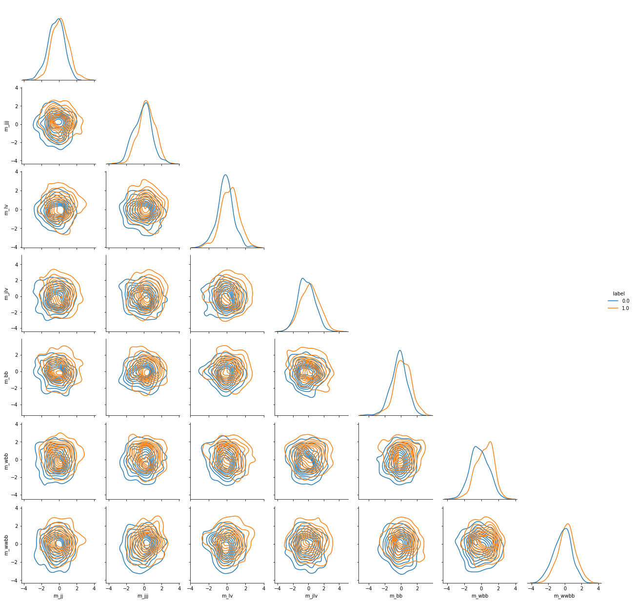
We can sample from this model, but it is untrained for now and gives random results.

def sample_to_pandas(sample_size):
    sam = d.sample(sample_size)
    fts = sam['features'].numpy()
    lbs = sam['labels'].numpy().astype('float32')
    dts = np.concatenate((fts, lbs), axis=1)
    names = column_labels[22:]
    names.append('label')
    return pd.DataFrame(dts, columns=names)

grid = sns.PairGrid(sample_to_pandas(500),
                    hue='label',
                    vars=column_labels[22:],
                    corner=True)
grid.map_diag(sns.kdeplot)
grid.map_offdiag(sns.kdeplot)
grid.add_legend()

<seaborn.axisgrid.PairGrid at 0x7f27de65e770>

Training

We go on training the algorithm on train dataset. We also check for the loss on validation samples.

accuracy = metrics.BinaryAccuracy()

def update_accuracy():
    """
    util function to update the binary accuracy metric
    to evaluate the algorithm performances.
    """
    accuracy.reset_state()
    y_true = test_dict['labels']
    y_pred, y_var, grad = d(test_dict['features'])
    accuracy.update_state(y_true, y_pred)
    return accuracy.result().numpy()

NUM_EPOCHS = 2
LR = 3e-4

weight = 1./NUM_FEATURES

history = {'accuracy': [], 'train_loss': [], 'val_loss': []}

trnl = 0.
vall = 0.
accu = 0.

learning_rate = tf.Variable(LR, trainable=False)
optimizer = tf.keras.optimizers.Adam(learning_rate)

print('+---------------+---------------+---------------+---------------+')
print('| EPOCH         | TRAIN_LOSS    | VAL_LOSS      | ACCURACY      |')
print('+---------------+---------------+---------------+---------------+')
for epoch in range(NUM_EPOCHS):
    for i, batch in enumerate(train_ds):
        trnl = train_step(optimizer, batch, weight)
        history['train_loss'].append(trnl)
        vall = -tf.reduce_mean(d.weighted_log_prob(val_dict, scaling_const=weight))
        history['val_loss'].append(vall)
        accu = update_accuracy()
        history['accuracy'].append(accu)
        print(f'| {epoch+1}, batch {i+1}\t| {trnl:.3f}    \t| {vall:.3f}    \t| {accu:.3f} \t|', end='\r')
    print(f'| {epoch+1}        \t| {trnl:.3f}    \t| {vall:.3f}    \t| {accu:.3f}   \t|')
print('+---------------+---------------+---------------+---------------+')

+---------------+---------------+---------------+---------------+
| EPOCH         | TRAIN_LOSS    | VAL_LOSS      | ACCURACY      |
+---------------+---------------+---------------+---------------+
| 1             | 0.339         | 0.319         | 0.665         ||
| 2             | 0.274         | 0.239         | 0.678         ||
+---------------+---------------+---------------+---------------+

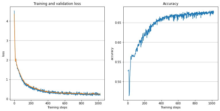
Results

To illustrate the results of the training, we plot the loss and accuracy history.

plt.figure(figsize=(13, 6))
plt.subplot(121)
plt.title('Training and validation loss')
plt.plot(history['train_loss'][1:], label='train loss')
plt.plot(history['val_loss'][1:], label='val loss')
plt.xlabel('Training steps')
plt.ylabel('loss')
plt.grid(axis='y')

# accuracy plot
plt.subplot(122)
plt.title('Accuracy')
plt.plot(history['accuracy'][1:])
plt.xlabel('Training steps')
plt.ylabel('accuracy')
plt.grid(axis='y')

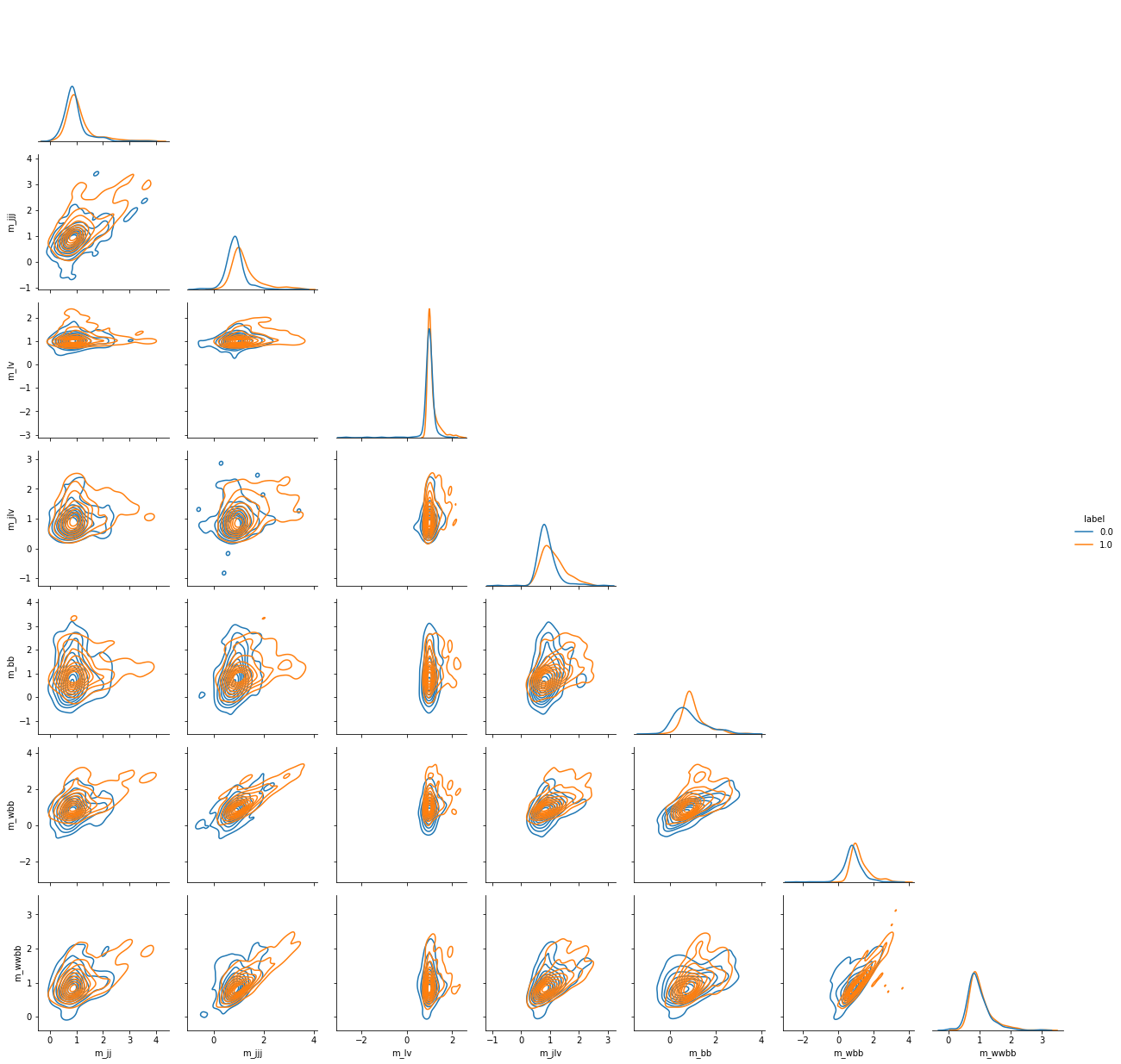
Now samples from our model are distributed accordingly to data.

grid = sns.PairGrid(sample_to_pandas(500),
                    hue='label',
                    vars=column_labels[22:],
                    corner=True)
grid.map_diag(sns.kdeplot)
grid.map_offdiag(sns.kdeplot)
grid.add_legend()

<seaborn.axisgrid.PairGrid at 0x7f2784475e70>