DIGLM Tutorial

In this notebook we illustrate with a toy model the usage of the DIGLM class.

The notebook is organized as follows:

1. Introduction;

2. Creation of a toy dataset;

3. Building the model and defining training functons;

4. Support function for plotting and sampling;

5. Training;

6. Results and final considerations

1. Introduction

An object of the DIGLM class is a trainable model which allows to accomplish the two following tasks:

1. Reproduce the feature distribution thanks to a normalizing flow step mapping the features to a latent space with multivariate normal distribution features;

2. Perform regression (linear, logistic and much more) with a Generalized Linear Model (GLM).

The idea comes from the article by E. Nalisnick et al. where the DIGLM model and algorithm characteristics is described and test on some examples are provided.

The two parts that constitute the algorithm are trained in a single feed-forward step of a semi-supervised training: given the features observation $ {x}_i ^N $ and their true labels $ {y}_i ^N $, the loss function minimized is

\begin{equation} - \sum_i \log{p(y|x; \theta, \beta)} + \lambda \log{p(x; \theta)} \end{equation}

where:

1. \(\beta\) are the weights of the glm;

2. \(\theta\) are the parameters that maps the distibution of \(x\) to the space of the latent variables \(z\) through the normalizing flow. The distribution of \(z\) is set to be a multivariate normal distribution with dimension equal to the space of the feature vectors;

3. \(\lambda\) is a hyper-parameter which weights the importance in the training of the two different parts of the loss: the first term indeed is used to solve the regression problem; the second one trains the normalizing flow.

import sys
sys.path.append('../../../src')
import os
import logging

import tensorflow as tf
from tensorflow import Variable, ones, zeros
from tensorflow_probability import glm
from tensorflow_probability import distributions as tfd
from tensorflow.keras import metrics
import numpy as np
import seaborn as sns
import sklearn.datasets as skd # where we can find a simple example
import matplotlib.pyplot as plt
import pandas as pd

from diglm import Diglm
from spqr import NeuralSplineFlow as NSF


# sinlencing tensorflow warnings
os.environ['TF_CPP_MIN_LOG_LEVEL'] = '3'
logging.getLogger('tensorflow').setLevel(logging.FATAL)

Cloning into 'diglm'...
remote: Enumerating objects: 828, done.
remote: Counting objects: 100% (220/220), done.
remote: Compressing objects: 100% (76/76), done.
remote: Total 828 (delta 169), reused 162 (delta 144), pack-reused 608
Receiving objects: 100% (828/828), 10.93 MiB | 3.40 MiB/s, done.
Resolving deltas: 100% (476/476), done.

2. Toy dataset

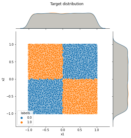
The feature vectors \(x_1\) and \(x_2\) are sampled from a uniform distribution \(U[-1, 1]\). The response function \(y(x_1, x_2): \mathbb{R}^2 \rightarrow \{0, 1\}\) is: $

\begin{cases} 1 \text{ if } x_1 \cdot x_2 > \dfrac{1}{x_1 \cdot x_2} \\ 0 \text{ elsewise} \\ \end{cases}

$

The sampled vectors and the response are transformed to a tf.data.Dataset.

#response function
response = lambda x1, x2: x1 * x2 > 1 / (x1 * x2)

BATCH_SIZE = 1024
DATASET_SIZE = BATCH_SIZE * 32
VAL_SIZE = BATCH_SIZE * 16

# dataset for training
X1 = np.random.uniform(low=-1, high=1, size=DATASET_SIZE)
X2 = np.random.uniform(low=-1, high=1, size=DATASET_SIZE)
df = pd.DataFrame(np.stack((response(X1, X2), X1, X2), axis=1),
                  columns=['labels','x1', 'x2'])

# dataset for validation
X1_val = np.random.uniform(low=-1, high=1, size=VAL_SIZE)
X2_val = np.random.uniform(low=-1, high=1, size=VAL_SIZE)
df_val = pd.DataFrame(np.stack((response(X1_val, X2_val), X1_val, X2_val), axis=1),
                  columns=['labels','x1', 'x2'])

# dataset for test
X1_test = np.random.uniform(low=-1, high=1, size=VAL_SIZE)
X2_test = np.random.uniform(low=-1, high=1, size=VAL_SIZE)
df_test = pd.DataFrame(np.stack((response(X1_test, X2_test), X1_test, X2_test), axis=1),
                  columns=['labels','x1', 'x2'])

# plotting the toy dataset with marginalized feature distribution too
joint_plot = sns.jointplot(data=df, x='x1', y='x2', hue='labels')
joint_plot.figure.suptitle('Target distribution', y = 1.05)

Text(0.5, 1.05, 'Target distribution')

3. Utilities: transforming datasets, sampling of distributions and plotting

We define some functions to transform our data into TesnorFlow datasets for automatic batching and parallelization; to extract sample from the transformed distributions and to plot them.

def to_tf_dataset(df, columns, dtype='float32', batch_size=32):
    """
    util function to transform a pandas.DataFrame into a
    batched tf.data.Dataset.

    """

    tf_ds = tf.data.Dataset.from_tensor_slices(df[columns].astype(dtype))
    tf_ds = tf_ds.prefetch(tf.data.experimental.AUTOTUNE)
    tf_ds = tf_ds.cache()
    tf_ds = tf_ds.batch(batch_size)
    return tf_ds

def sampling(size=500):
    """
    returns a sample of the transformed disribution and its computed
    response through glm evaluation.

    """
    trans_sample = diglm.sample(size)['features']
    mean_sample, var_sample, grad_sample  = diglm(trans_sample)
    x1, x2 = np.split(trans_sample.numpy(), 2, axis=1)
    x1 = np.concatenate(x1)
    x2 = np.concatenate(x2)
    mean = np.concatenate(mean_sample.numpy().T)
    return mean, x1, x2

def plot(name, counter=None):
    """
    plotting function that gets some samples from the norm. flow
    inverse distribution and the calculated response and plots it
    alongside with the target distribution
    """
    # Get sampling data to plot
    mean, x1, x2 = sampling(size=VAL_SIZE)
    df_train = pd.DataFrame(np.stack((mean, x1, x2), axis=1),
                            columns=['labels', 'x1', 'x2'])
    #plot
    ax_1 = sns.scatterplot(data=df_train, x='x1', y='x2', hue='labels', palette='coolwarm')
    ax_1.set_ylim(min(x1), max(x1))
    ax_1.set_xlim(min(x1), max(x2))
    if counter is not None: # used to track the training epoch
        ax_1.set_title(f'Training epoch = {counter}')

    plt.savefig(name)

train_ft = to_tf_dataset(df, ['x1', 'x2'], batch_size=BATCH_SIZE)
train_l = to_tf_dataset(df, ['labels'], dtype='int32', batch_size=BATCH_SIZE)

val_ft = to_tf_dataset(df_val, ['x1', 'x2'], batch_size=VAL_SIZE)
val_l = to_tf_dataset(df_val, ['labels'], dtype='int32', batch_size=VAL_SIZE)

test_ft = to_tf_dataset(df_test, ['x1', 'x2'], batch_size=VAL_SIZE)
test_l = to_tf_dataset(df_test, ['labels'], dtype='int32', batch_size=VAL_SIZE)

4. Building the DIGLM

We initialize our diglm model with:

1. a NeuralSplineFlow object as bijector with two splits (there are only two variables

2. a tf.glm.Bernoulli() as glm to realize the logistic regression.

my_glm = glm.Bernoulli()
neural_spline_flow = NSF(splits=2, spline_params=dict())
diglm = Diglm(neural_spline_flow, my_glm, 2)

train_dict = [{'labels': batch_l,
              'features': batch_ft}
              for batch_l, batch_ft in zip(train_l, train_ft)]
val_dict = [{'labels': batch_l,
              'features': batch_ft}
              for batch_l, batch_ft in zip(val_l, val_ft)]
test_dict = [{'labels': batch_l,
              'features': batch_ft}
              for batch_l, batch_ft in zip(test_l, test_ft)]


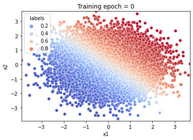
# let's visualize a sample from the inverse distribution of the bijector
# before training.
plot('start.jpeg', counter=0)

5. Training

First, we define a train step, where the loss and its gradient are calculated and the training variables of the model are updated accordingly. We follow the keras tutorial.

@tf.function
def train_step(optimizer, target_sample, weight=.1):
    """
    Train step function for the diglm model. Implements the basic steps for computing
    and updating the trainable variables of the model. It also
    calculates the loss on training and validation samples.

    """

    with tf.GradientTape() as tape:
        # calculating loss and its gradient of training data
        loss = -tf.reduce_mean(diglm.weighted_log_prob(target_sample, scaling_const=weight))
    variables = tape.watched_variables()
    gradients = tape.gradient(loss, variables)
    optimizer.apply_gradients(zip(gradients, variables))
    return loss

Now we are ready to train the model!

# we define a suitable metric
accuracy = metrics.BinaryAccuracy()

def update_accuracy():
    """
    util function to update the binary accuracy metric
    to evaluate the algorithm performances.
    """
    accuracy.reset_state()
    y_true = test_dict[0]['labels']
    y_pred, y_var, grad = diglm(test_dict[0]['features'])
    accuracy.update_state(y_true, y_pred.numpy())
    history['accuracy'].append(accuracy.result().numpy())

# hyper parameters
LR = 5e-3
NUM_EPOCHS = 500
learning_rate = tf.Variable(LR, trainable=False)
optimizer = tf.keras.optimizers.Adam(learning_rate)

loss = 0
val_loss = 0
history = {'accuracy': [], 'train_loss': [], 'val_loss': []}
fig_list = []

weight = 1

update_accuracy()
print(accuracy.result().numpy())

# training loop on epochs
for epoch in range(NUM_EPOCHS):
    if epoch == int(NUM_EPOCHS / 2):
        weight = 0.5
    if epoch % 10 == 0:
        # plot
        name = f'fig{epoch}.jpeg'
        fig_list.append(name)
        plot(name, counter=(epoch + 1))
        plt.close()
        print(f'Epoch = {epoch+1} \t Loss = {loss:.3f} \t Val loss = {val_loss:.3f}')
    # train batch per batch
    for train_batch, val_batch in zip(train_dict, val_dict):
        loss = train_step(optimizer, train_batch, weight=weight)
        # validation loss
        val_loss = -tf.reduce_mean(diglm.weighted_log_prob(val_batch, scaling_const=weight))
        # updating loss and accuracy
        update_accuracy()
        history['train_loss'].append(loss)
        history['val_loss'].append(val_loss)

0.49371338
Epoch = 1        Loss = 0.000    Val loss = 0.000
Epoch = 11       Loss = 2.908    Val loss = 2.868
Epoch = 21       Loss = 2.808    Val loss = 2.910
Epoch = 31       Loss = 2.614    Val loss = 2.814
Epoch = 41       Loss = 2.413    Val loss = 2.779
Epoch = 51       Loss = 2.422    Val loss = 2.807
Epoch = 61       Loss = 2.324    Val loss = 2.676
Epoch = 71       Loss = 2.400    Val loss = 2.614
Epoch = 81       Loss = 2.252    Val loss = 2.629
Epoch = 91       Loss = 2.161    Val loss = 2.480
Epoch = 101      Loss = 2.108    Val loss = 2.503
Epoch = 111      Loss = 2.052    Val loss = 2.484
Epoch = 121      Loss = 2.043    Val loss = 2.426
Epoch = 131      Loss = 2.106    Val loss = 2.431
Epoch = 141      Loss = 2.046    Val loss = 2.455
Epoch = 151      Loss = 1.982    Val loss = 2.369
Epoch = 161      Loss = 1.975    Val loss = 2.333
Epoch = 171      Loss = 1.969    Val loss = 2.400
Epoch = 181      Loss = 1.915    Val loss = 2.365
Epoch = 191      Loss = 1.904    Val loss = 2.309
Epoch = 201      Loss = 1.863    Val loss = 2.310
Epoch = 211      Loss = 1.842    Val loss = 2.255
Epoch = 221      Loss = 1.884    Val loss = 2.220
Epoch = 231      Loss = 1.847    Val loss = 2.205
Epoch = 241      Loss = 1.908    Val loss = 2.248
Epoch = 251      Loss = 1.821    Val loss = 2.231
Epoch = 261      Loss = 1.087    Val loss = 1.300
Epoch = 271      Loss = 1.042    Val loss = 1.261
Epoch = 281      Loss = 1.031    Val loss = 1.249
Epoch = 291      Loss = 1.072    Val loss = 1.222
Epoch = 301      Loss = 1.048    Val loss = 1.244
Epoch = 311      Loss = 1.012    Val loss = 1.217
Epoch = 321      Loss = 0.976    Val loss = 1.199
Epoch = 331      Loss = 1.046    Val loss = 1.176
Epoch = 341      Loss = 0.987    Val loss = 1.207
Epoch = 351      Loss = 1.004    Val loss = 1.149
Epoch = 361      Loss = 0.981    Val loss = 1.146
Epoch = 371      Loss = 0.969    Val loss = 1.130
Epoch = 381      Loss = 0.959    Val loss = 1.189
Epoch = 391      Loss = 0.947    Val loss = 1.109
Epoch = 401      Loss = 0.930    Val loss = 1.101
Epoch = 411      Loss = 0.914    Val loss = 1.091
Epoch = 421      Loss = 0.958    Val loss = 1.091
Epoch = 431      Loss = 1.025    Val loss = 1.075
Epoch = 441      Loss = 0.916    Val loss = 1.083
Epoch = 451      Loss = 0.927    Val loss = 1.077
Epoch = 461      Loss = 0.888    Val loss = 1.067
Epoch = 471      Loss = 0.903    Val loss = 1.094
Epoch = 481      Loss = 0.918    Val loss = 1.080
Epoch = 491      Loss = 0.891    Val loss = 1.048

6. Results

To illustrate the results of the training, we plot:

1. a gif illustrating how the algorithm learnt both to reproduce the feature distribution and the response

2. The loss and accuracy history

from plot_utils import make_gif


make_gif(fig_list, "diglm_example.gif", duration=0.3)

# loss plot
plt.figure(figsize=(13, 6))
plt.subplot(121)
plt.title('Training and validation loss')
plt.plot([i for i in range(len(history['train_loss'])-1)],
        history['train_loss'][1:],
        label='train loss')
plt.plot([i for i in range(len(history['val_loss'])-1)],
        history['val_loss'][1:],
        label='val loss')
plt.xlabel('Training steps')
plt.ylabel('loss')
plt.vlines([250], 1, 3.7, color='red')
plt.text(180, 3.5, r'$\lambda$ = 1.     $\lambda$ = 0.5')
plt.grid(axis='y')

# accuracy plot
plt.subplot(122)
plt.title('Accuracy')
plt.plot([i for i in range(len(history['accuracy']))],
        history['accuracy'])
plt.xlabel('Training steps')
plt.ylabel('accuracy')
plt.vlines([250], 0.35, 0.95, color='red')
plt.text(190, 0.4, r'$\lambda$ = 1.   $\lambda$ = 0.5')
plt.grid(axis='y')

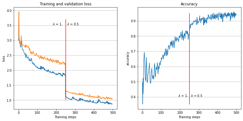
Referring to the gif, we see that the algorithm accomplished the task of evaluating the dataset feature distribution as well as the response function. The quality of the response evaluation is monitored through the BinaryAccuracy metric, counting the fraction:

\begin{equation} \dfrac{\text{True Positive}}{\text{True Positive + False Negative}} \end{equation}

where the Positive / Negative cut on the response function is set to 0.5. After 500 epochs, the loss function attains a plateau and the accuracy is stably around 0.94.

Just as in the SpQR notebook, we can evaluate the quality of the feature distribution evaluation using a Kolmogorov-Smirnov test

from scipy.stats import ks_2samp


#slicing and preparing arrays to perform the test
mean, x1_trans, x2_trans = sampling(1000)
mean_target, x1_target, x2_target = np.squeeze(np.split(df.to_numpy(), 3, axis=1))

# calculating statistic from K-S test and p-values
stat_1, pval_1 = ks_2samp(x1_trans, x1_target)
stat_2, pval_2 = ks_2samp(x2_trans, x2_target)

print(f'p-value x1 distribution = {pval_1}')
print(f'p-value x2 distribution = {pval_2}')

p-value x1 distribution = 0.00026182909606191183
p-value x2 distribution = 0.00020538468989076796

We see that in this DIGLM model the capability of the algorithm to learn the univariate distributions of the features \(x_1\) and \(x_2\) is reduced with respect to the pure NeuralSplineFLow model (and we can expect it to be also less accurate in prediction than the simple GLM model). That’s because the algorithm tries to minimize the loss on a wider parameter space.

About \(\lambda\)

The hyper-parameter \(\lambda\) weights the two component of the log-likelihood loss, favouring the training of one part of the algorithm over the other. In middle of the training we switched it from 1 to 0.5: this resulted of course in a diminution of the likelihood, but what’s interesting to notice is that the binary accuracy atteined rapidly a better result after the diminution, just as stated in the article. To obtain pure predictive or pure generative model it is sufficient to set \(\lambda\) to very high (or very low) value (with respect to 1.).